Understanding Machine Learning

Machine Learning is tough if you haven’t been there from the beginning because the ecosystem is rapidly developing and growing. In a world with access to a lot of data and a lot of compute, Machine Learning, an idea to teach machine from examples and experience - without being explicitly programmed, perfectly makes sense.

This is in a draft version.

When I started learning and reading about machine learning I came across this definition:

Machine learning is a field of artificial intelligence that uses statistical techniques to give computer systems the ability to “learn” (e.g., progressively improve performance on a specific task) from data, without being explicitly programmed.

I always struggled to understand “progressively improve performance on a specific task”. Of course, there is some programing involved. How can a computer algorithm be generic enough to “learn” from any data. What about the deterministic behaviour of computer algorithms?

The goal of this article is to provide a little context on:

how the modern machine learning algorithms have grown
why machine learning is a good technique for many different applications and domains
why machine learning works (e.g., why a machine learns)

For this introduction to machine learning, We will go through a toy example of curve fitting problem. We will first approach this problem using elementary algebra, the “old school” way, then we will solve it using machine learning with two different algorithms.

Curve Fitting

We want to learn a function f(x) which maps the input x to the output y. For simplicity in this example let x,y belong to the set of real number R.

Lets say we are given sample observations as follows:

x	y = f(x)
1	21
2	53
3	101
4	165

Our goal is to learn a function that maps points as best as possible. Once we learn this function we would be able to predict ŷ for any new input x.

Learning in this context means:

to be able to fit the data to find relationships with various inputs
to be able to predict output for new input value

If this mapping was similar to the step function like mapping, we could learn what is the best threshold value to always be on one side of the function output. Predicting output for a given input is a powerful tool, because we can apply that to many functions in different applications.

Of course, here we assumed that the function accepts single real number input and produces a single real number output. (We will discuss about this later.)

Solving with Algebra

The method below is described from an online lecture. For more information you can check here

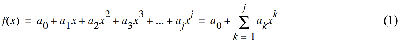
Let’s assume that the function f(x) is a polynomial of degree j:

polynomial

unknowns

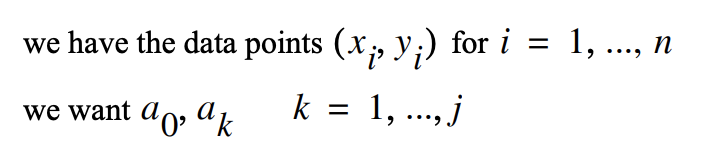
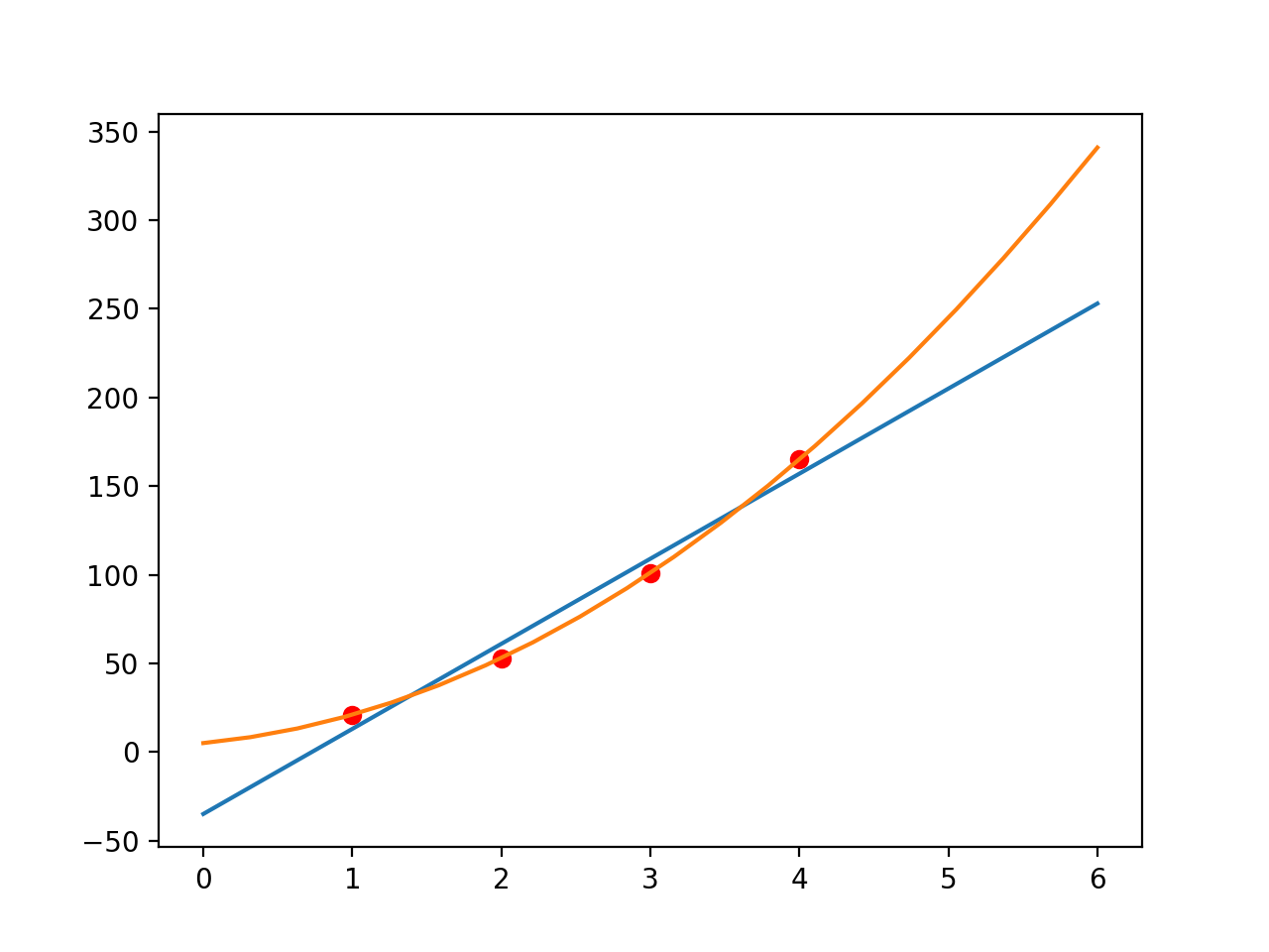
Let’s plot the data points we have:

points

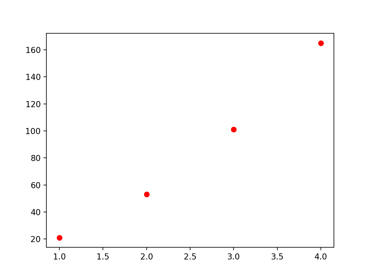
When we try to fit these points with a line: we want to know the function that represents a line which would look like this:

1st-order-curve

Because these are only 4 data points we get a feeling that the data is linear and we may be able to fit in the first order polynomial. But in fact the data is generated from the second order function. Original points belonged to the equation y = 8*x^2 + 8*x + 5

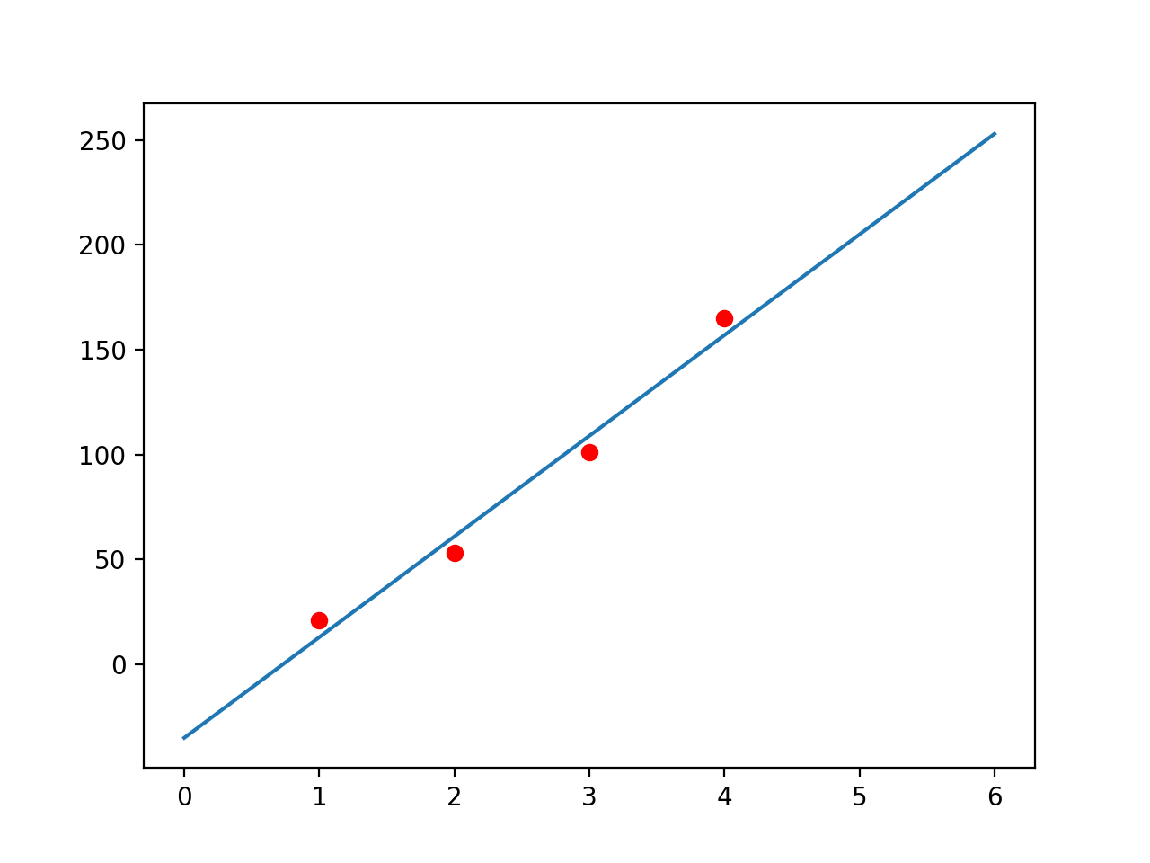
So these would fit nicely when we try to with to second order polynomial:

2nd-order-curve

We can compute the function based on the formula of least squared approach - and minimize that function with respect to the coefficients we want to find to best “fit” our data points.

solution

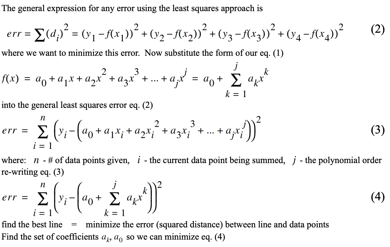
If last part is complex then ignore - it just sums up one metric about the function we know from all the data points we have. That computed metric is known as the error. (In this particular case error is computed using sum of squared of differences.)

After this to find the parameters(coefficients) which minimises this error metric; we take derivatives of error with respect to the coefficients. (minimum error => derivative is zero.) We can put those derivative equations in matrix and solve using linear algebra. The code for this looks like below:

From this approach we are able to get the coefficients of the polynomial. And able to fit the data to the function. Once we learned these coefficients we would also be able to predict output for new input.

However, there are issues with this approach:

If you looked in the code snippet - at one point it had to compute matrix inverse in order to solve the linear algebra system. That is computationally in-efficient and also not guaranteed to be possible in all cases. And becomes non-trivial with more number of coefficients.
We have figure out value of the order j.
Always assumes that the relationship of function is linear. (Which is ok, based on how we defined our curve fitting problem, but actually not all functions are having linear relationship - we want to remove this assumption now.)

Lets try to approach above issues with two different approach in machine learning, applying to the same problem.

Solving with Gradient Descent Optimizer

We are going to derive inspiration of error from linear algebra. We want to minimize that error to fit our data points. But we assume that here, we have many data points available for our functions. So imagine that rather having only four points for the (x,y) entry in the table we have say 10k of them from the same function. (This is the case for many real world example for machine learning tasks where we want to learn complex functions but have huge data set backing the mapping). However, we want to avoid matrix inverse operation.

Ignore the parts you are not able to understand about underlying framework details - but notice following things:

it assume random initial states of the coefficients
it looks at all the data points and computes the error
performs gradient optimization (compute derivatives) in the direction of minimizing the error
updates coefficients with the learning rate
repeats this as many time as needed until convergence

Benefits of above approach:

In above code we have removed the constraint on order of the polynomial. The order j is also learned.
The gradient technique is so powerful that we can change the mapping y to other function of x and it would still fit in that.
We could also make y depend on more than one input params. So now our function could be accepting more that one features. (x1, x2, … so on)

What does it learn

This is the loss per iterations of the training:

tf-loss-plot

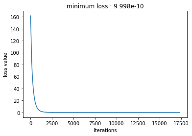
After 17335 Iterations it learns that the Equation is: y = 8.001574x^1.9997478723526 + 7.998249530792236x + 5.0001220703125.

Above algorithm is generic enough to work well with many different machine learning technique, And it is perfectly good technique to use in many real world problems! However there are still following improvements we could make:

We still have to define the mapping y to some function of x with coefficients (parameters). (e.g., we defined y to be polynomial of x in above code)
Above step requires hand-engineering to perform feature analysis and put mapping with appropriate relations with dependent features. So called feature engineering.
The relationship of function is still linear combination of the input features.

Solving with Neural Network

We make improvements to gradient optimization and use neural network, a generic framework build upon combining many neurons, an inspiration from how a human brain might learn anything. Any function we want to learn is the combination of many connected layers (deep) and each layers is set of neurons. That is why this technique is called deep learning. Each neuron has an input and its own parameters governing whether to be active on the input.

Benefits of above approach:

Notice here we are not specifying anything about function being polynomial. Function is just combination of neuron layers.
No feature engineering needed because it learns that.
Non-linearity is added in each neuron computation based on which a neuron decides to activate itself.
We can model complex functions with as many as millions of parameters to learn by increasing the number of layers and the number of neurons in each layer.

What does it learn

This is the loss per iterations of the training:

nn-loss-plot

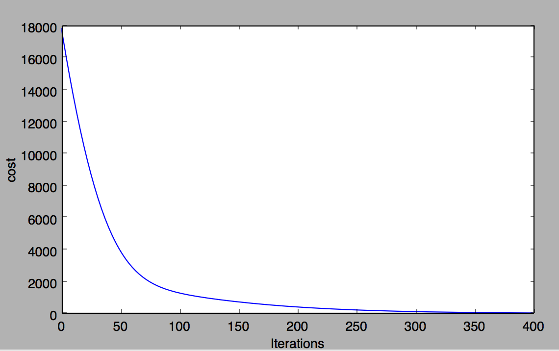
Above code is generic enough that it does not consider any assumption of polynomial’s order. In fact you can try creating a sample data from any other degree of polynomial and feed that in the network and it would learn the mapping for that fitting. (for higher order than 5 we need to make the the network deeper than just 2 layers maybe.) And it would be able to predict the correct value for the new input.

However, how big (number of layers and neurons) our network should be, for a given problem becomes a tuning task. We have to experiment and judge. Along with this, there will be many hyper-parameters we need to tune in case of deep-learning neural network. Interesting research is happening in this area to develop tools for hyperparameters tuning, and also model new neuron units for a specific task. (for e.g., convolution neuron for image classification related tasks)

Why learning is feasible?

Interesting thinking is why above techniques actually work. Learning is used when a. A pattern exists b. We can not pin it down mathematically c. We have data on it. The last part is essential. The learning problem explained above can be described (for all three cases) formally as follows:

We have unknown target y = f(x) We have data set (x1, y1), (x2, y2), … (xN, yN) Learning algorithm picks a function g ~ f from the hypothesis set H

Hopefully g approximates f.

The answer of this hope is that learning is derived from a probabilistic situation.

Theory of learning

This is where probability would help.

In science and in engineering, you go a huge distance by settling for not absolutely certain, but almost certain. - Prof. Yaser Abu-Mostafa

Let say you have a bin with infinite marbles. And a marble can be either red of green.

Hence picking up a marble randomly from the bin and it happening to be red has some probability. Let say that probability is π. Therefore, probability of marble being green is: 1 - π.

π is unknown.

Consider a sample of N marbles picked from the bin. What does the fraction (λ) of red marbles in that samples, in-sample frequency, could tell you about the original probability π,_ out-sample frequency_? (say p marbles are red and N-p are green in the sample. => λ=p/(N-p).)

This is the analogy of our learning problem.

One sample could not convey information about actual π certainly. But many such samples and with bigger N (large N), statistics tells us that, this fraction would likely be close to π (within ε) with almost certainty. Why? Law of large numbers.

Hoeffding’s inequality provides an upper bound for probability being farther its expected value. (Formally, probability P[|λ-π| > ε] is bounded. - we can ignore the mathematics machinery of Hoeffding’s for this post)

Which in our case would state that λ = π is probably approximately correct.

Lets add probability to your input sample data. The sample data set came from distribution, whether you like it or not.
There exists is a probability distribution of picking one point vs another of the input space of the unknown target function (x1, x2, …)
Let it be any distribution so any probability for picking a point x. (Because the Hoeffding bound, which is a negative exponential of ε, does not depend on λ or π.)
But if we add this assumption our learning problem’s algorithms error is bounded by Hoeffding’s inequality.

That is saying that the in-sample frequency can model the out-sample frequency. This is where we are generalizing the learning.

That means learning from the sample of the data set, we can generalize the learning of function for whole input data space.

This by no means conveys that all learned model from in-sample data set is generic enough for out-sample data, there are still many problems we have to deal with like, overfit, underfit, exploding gradients, etc. But it conveys that it is feasible.

Acknowledgement

Thanks to Noman and Shubham for providing their solutions of curve fitting scripts.

Curve Fitting

Solving with Algebra

Solving with Gradient Descent Optimizer

What does it learn

Solving with Neural Network

What does it learn

Why learning is feasible?

Theory of learning

Acknowledgement

References: